The import thing behind DDPM

The short summary will divide into three part, the first part show the model and the detail. the second part show the things behind the model. The third part show the thinking about GAN and further.

detail of DDPM model

Forward process

前向扩散过程：给定一个从分布中取样的数据点$x_0\sim p(x_0)$，前向扩散过程就是指分步向样本添加少量的高斯噪声，产生一连串的噪声样本，步长由方差${\beta_t \in (0,1) }_{t=1}^t$来控制：

$q(x_{1:T}

x_0) \coloneqq \prod_{t=1}^{T}q(x_t

x_{t-1})$

$q(x_t

x_{t-1}) \coloneqq \mathcal N(x_t; \sqrt{1-\beta_t} x_{t-1},\beta_t\textbf{I})$

当 $T\to\infty$, $x_t$等效于各向同性的高斯分布。

前向过程的一个特点是它允许在任意时间$t$对 $x_t$ 进行采样: 此处用到了reparameterization trick. 记$\alpha_t =1-\beta_t$, $\bar{\alpha_t} = \prod_{i=1}^T\alpha_i$:

\[\begin{aligned} x_t &= \sqrt{\alpha_t}x_{t-1} + \sqrt{1-\alpha_t}z_{t-1} \\ &=\sqrt{\alpha_t\alpha_{t-1}}x_{t-2} + \sqrt{1-\alpha_t\alpha_{t-1}}\overline{z_{t-2}} \\ & = \sqrt{\bar{\alpha_t}}x_0+\sqrt{1-\bar{\alpha_t}}z\\ \end{aligned}\]

这里$z_i\coloneqq \mathcal N(0,\textbf{I})$, 而 $\overline{z_{t-2}}$是两个具有不同方差的高斯相加时后的表示 :$\sqrt{(1-\alpha_t) + \alpha_t(1-\alpha_{t-1})} = \sqrt{1-\alpha_t\alpha_{t-1}}$

**所以有 $q(x_t

x_0) = \mathcal N(x_t,\sqrt{\bar{\alpha_t}}x_0,\sqrt{1-\bar{\alpha_t}}\textbf{I})$**

Reverse process

如果我们可以反转上述过程，也就是说从$x_T \coloneqq \mathcal N(\textbf{0},\textbf{1})$中得到原本的sample，问题就能解决了。

这里不太确定？受Bayesian Learning via Stochastic Gradient Langevin Dynamics启发，原始雏形中运用了Stochastic Gradient Langevin Dynamics的方法进行采样。

但是由于$q(x_{t-1}

x_{t})$是未知的，所以我们需要得到一个$p_\theta$来近似，所以关键任务就是需要学习来逼近反向扩散过程中的条件概率分布：

$p_\theta(x_{0:T}) = p(x_T)\prod_{t=1}^Tp_\theta(x_{t-1}	x_t)$
$p_\theta(x_{t-1}	x_t) \coloneqq \mathcal N(x_{t-1}; \mu_\theta(x_t,t), \Sigma_\theta(x_t,t))$

国际惯例，使用变分下限来优化负对数似然。通过最小化损失，我们最大化了生成真实数据样本的概率的下限：

\[\begin{aligned} -\log p_\theta(\mathbf{x}_0) &\leq - \log p_\theta(\mathbf{x}_0) + D_\text{KL}(q(\mathbf{x}_{1:T}\vert\mathbf{x}_0) \| p_\theta(\mathbf{x}_{1:T}\vert\mathbf{x}_0) ) \\ &= -\log p_\theta(\mathbf{x}_0) + \mathbb{E}_{\mathbf{x}_{1:T}\sim q(\mathbf{x}_{1:T} \vert \mathbf{x}_0)} \Big[ \log\frac{q(\mathbf{x}_{1:T}\vert\mathbf{x}_0)}{p_\theta(\mathbf{x}_{0:T}) / p_\theta(\mathbf{x}_0)} \Big] \\ &= -\log p_\theta(\mathbf{x}_0) + \mathbb{E}_q \Big[ \log\frac{q(\mathbf{x}_{1:T}\vert\mathbf{x}_0)}{p_\theta(\mathbf{x}_{0:T})} + \log p_\theta(\mathbf{x}_0) \Big] \\ &= \mathbb{E}_q \Big[ \log \frac{q(\mathbf{x}_{1:T}\vert\mathbf{x}_0)}{p_\theta(\mathbf{x}_{0:T})} \Big] \\ \text{令 }L_\text{VLB} &= \mathbb{E}_{q(\mathbf{x}_{0:T})} \Big[ \log \frac{q(\mathbf{x}_{1:T}\vert\mathbf{x}_0)}{p_\theta(\mathbf{x}_{0:T})} \Big] \end{aligned}\]

推导于 Appendix A: Deep Unsupervised Learning using Nonequilibrium Thermodynamics)

\[\begin{aligned} L_\text{VLB} &= \mathbb{E}_{q(\mathbf{x}_{0:T})} \Big[ \log\frac{q(\mathbf{x}_{1:T}\vert\mathbf{x}_0)}{p_\theta(\mathbf{x}_{0:T})} \Big] \\ &= \mathbb{E}_q \Big[ \log\frac{\prod_{t=1}^T q(\mathbf{x}_t\vert\mathbf{x}_{t-1})}{ p_\theta(\mathbf{x}_T) \prod_{t=1}^T p_\theta(\mathbf{x}_{t-1} \vert\mathbf{x}_t) } \Big] \\ &= \mathbb{E}_q \Big[ -\log p_\theta(\mathbf{x}_T) + \sum_{t=1}^T \log \frac{q(\mathbf{x}_t\vert\mathbf{x}_{t-1})}{p_\theta(\mathbf{x}_{t-1} \vert\mathbf{x}_t)} \Big] \\ &= \mathbb{E}_q \Big[ -\log p_\theta(\mathbf{x}_T) + \sum_{t=2}^T \log \frac{q(\mathbf{x}_t\vert\mathbf{x}_{t-1})}{p_\theta(\mathbf{x}_{t-1} \vert\mathbf{x}_t)} + \log\frac{q(\mathbf{x}_1 \vert \mathbf{x}_0)}{p_\theta(\mathbf{x}_0 \vert \mathbf{x}_1)} \Big] \\ &= \mathbb{E}_q \Big[ -\log p_\theta(\mathbf{x}_T) + \sum_{t=2}^T \log \Big( \frac{q(\mathbf{x}_{t-1} \vert \mathbf{x}_t, \mathbf{x}_0)}{p_\theta(\mathbf{x}_{t-1} \vert\mathbf{x}_t)}\cdot \frac{q(\mathbf{x}_t \vert \mathbf{x}_0)}{q(\mathbf{x}_{t-1}\vert\mathbf{x}_0)} \Big) + \log \frac{q(\mathbf{x}_1 \vert \mathbf{x}_0)}{p_\theta(\mathbf{x}_0 \vert \mathbf{x}_1)} \Big] \\ &= \mathbb{E}_q \Big[ -\log p_\theta(\mathbf{x}_T) + \sum_{t=2}^T \log \frac{q(\mathbf{x}_{t-1} \vert \mathbf{x}_t, \mathbf{x}_0)}{p_\theta(\mathbf{x}_{t-1} \vert\mathbf{x}_t)} + \sum_{t=2}^T \log \frac{q(\mathbf{x}_t \vert \mathbf{x}_0)}{q(\mathbf{x}_{t-1} \vert \mathbf{x}_0)} + \log\frac{q(\mathbf{x}_1 \vert \mathbf{x}_0)}{p_\theta(\mathbf{x}_0 \vert \mathbf{x}_1)} \Big] \\ &= \mathbb{E}_q \Big[ -\log p_\theta(\mathbf{x}_T) + \sum_{t=2}^T \log \frac{q(\mathbf{x}_{t-1} \vert \mathbf{x}_t, \mathbf{x}_0)}{p_\theta(\mathbf{x}_{t-1} \vert\mathbf{x}_t)} + \log\frac{q(\mathbf{x}_T \vert \mathbf{x}_0)}{q(\mathbf{x}_1 \vert \mathbf{x}_0)} + \log \frac{q(\mathbf{x}_1 \vert \mathbf{x}_0)}{p_\theta(\mathbf{x}_0 \vert \mathbf{x}_1)} \Big]\\ &= \mathbb{E}_q \Big[ \log\frac{q(\mathbf{x}_T \vert \mathbf{x}_0)}{p_\theta(\mathbf{x}_T)} + \sum_{t=2}^T \log \frac{q(\mathbf{x}_{t-1} \vert \mathbf{x}_t, \mathbf{x}_0)}{p_\theta(\mathbf{x}_{t-1} \vert\mathbf{x}_t)} - \log p_\theta(\mathbf{x}_0 \vert \mathbf{x}_1) \Big] \\ &= \mathbb{E}_q [\underbrace{D_\text{KL}(q(\mathbf{x}_T \vert \mathbf{x}_0) \parallel p_\theta(\mathbf{x}_T))}_{L_T} + \sum_{t=2}^T \underbrace{D_\text{KL}(q(\mathbf{x}_{t-1} \vert \mathbf{x}_t, \mathbf{x}_0) \parallel p_\theta(\mathbf{x}_{t-1} \vert\mathbf{x}_t))}_{L_{t-1}} \underbrace{- \log p_\theta(\mathbf{x}_0 \vert \mathbf{x}_1)}_{L_0} ] \end{aligned}\]

顺达一提，2015中使用了Jensen不等式最小化交叉熵，也会得到一样的结果，最小实质上就是似然值最大。（？需要补充）

此时我们发现问题出现在$L_{t-1}$这一项：因为对$L_T$来说是个常量($X_T$是高斯分布)，$L_0$也好说。

但很快我们发现当基于$x_0$的时候，$q(x_{t-1}

x_t,x_0)$是很好表达的。运用贝叶斯公式：

\[\begin{aligned} q(x_{t-1}|x_t,x_0) &= q(x_t|x_{t-1},x_0)\frac{q(x_{t-1}|x_0)}{q(x_{t}|x_0)} \\ &\propto exp(-\frac{1}{2}(\frac{(x_t - \sqrt{a_t}x_{t-1})^2}{\beta_t}- \frac{(x_{t-1} - \sqrt{\bar{a_{t-1}}}x_0)^2}{1 - \bar{\alpha_{t-1}}} + \frac{(x_{t} - \sqrt{\bar{a_t}}x_0)^2}{1 - \bar{\alpha_{t}}} )) \\ & \propto Ax_{t-1}^2 + Bx_{t-1}+C\\ \end{aligned}\]

所以当基于$x_0$的时候，$q(x_{t-1}	x_t,x_0)$可以表示为：
$q(x_{t-1}	x_t,x_0) = \mathcal N(x_t-1;\tilde{\mu}(x_t,x_0),\tilde{\beta_t\textbf{I}})$

$\tilde{\beta}t = 1/(\frac{\alpha_t}{\beta_t} + \frac{1}{1 - \bar{\alpha}{t-1}}) = \frac{1 - \bar{\alpha}_{t-1}}{1 - \bar{\alpha}_t} \cdot \beta_t$

$\tilde{\mu}t (x_t, x_0) = (\frac{\sqrt{\alpha_t}}{\beta_t} x_t + \frac{\sqrt{\bar{\alpha}_t}}{1 - \bar{\alpha}_t} x_0)/(\frac{\alpha_t}{\beta_t} + \frac{1}{1 - \bar{\alpha}{t-1}}) = \frac{\sqrt{\alpha_t}(1 - \bar{\alpha}{t-1})}{1 - \bar{\alpha}_t}x_t + \frac{\sqrt{\bar{\alpha}{t-1}}\beta_t}{1 - \bar{\alpha}_t} x_0$

recall我们在向前扩散的时候我们得到了：

$x_t = \sqrt{\bar{\alpha_t}}x_0+\sqrt{1-\bar{\alpha_t}}z_t$

将$x_0$替换带入后有：

$\tilde{\mu_t} = \frac{1}{\sqrt{\alpha_t}}(x_t - \frac{\beta_t}{\sqrt{1-\bar{\alpha_t}}}z_t)$

所以现在的情况是：

我们需要训练$\mu_\theta$去predict $\tilde{\mu_t} = \frac{1}{\sqrt{\alpha_t}}(x_t - \frac{\beta_t}{\sqrt{1-\bar{\alpha_t}}}z_t)$

由于$x_t$在训练的时候是输入项, 所以我们reparameterize$z_\theta$:

$\mu_\theta(x_t,t) = \frac{1}{\sqrt{\alpha_t}}(x_t - \frac{\beta_t}{\sqrt{1-\bar{\alpha_t}}}z_\theta(x_t,t))$

所以

$x_{t-1} = \mathcal{N}(x_{t-1}; \frac{1}{\sqrt{\alpha_t}} \Big( x_t - \frac{\beta_t}{\sqrt{1 - \bar{\alpha}t}} z\theta(x_t, t) \Big), \boldsymbol{\Sigma}_\theta(x_t, t))$

(注意sampling的准则出现了)

根据$D_{KL}$的定义, $L_t$这一项就可以改写为：

$L_{t-1} = \mathbb{E}{\mathbf{x}_0, \mathbf{z}} \Big[\frac{1}{2 | \boldsymbol{\Sigma}\theta(\mathbf{x}t, t) |^2_2} | {\tilde{\boldsymbol{\mu}}_t(\mathbf{x}_t, \mathbf{x}_0)} - {\boldsymbol{\mu}\theta(\mathbf{x}_t, t)} |^2 \Big] + C$

其中C为与$\theta$无关的常数

所以

\[\begin{aligned} L_{t-1} - C &= \mathbb{E}_{\mathbf{x}_0, \mathbf{z}} \Big[\frac{1}{2 \|\boldsymbol{\Sigma}_\theta \|^2_2} \| {\frac{1}{\sqrt{\alpha_t}} \Big( \mathbf{x}_t - \frac{\beta_t}{\sqrt{1 - \bar{\alpha}_t}} \mathbf{z}_t \Big)} - {\frac{1}{\sqrt{\alpha_t}} \Big( \mathbf{x}_t - \frac{\beta_t}{\sqrt{1 - \bar{\alpha}_t}} \boldsymbol{\mathbf{z}}_\theta(\mathbf{x}_t, t) \Big)} \|^2 \Big] \\ &= \mathbb{E}_{\mathbf{x}_0, \mathbf{z}} \Big[\frac{ \beta_t^2 }{2 \alpha_t (1 - \bar{\alpha}_t) \| \boldsymbol{\Sigma}_\theta \|^2_2} \|\mathbf{z}_t - \mathbf{z}_\theta(\mathbf{x}_t, t)\|^2 \Big] \\ &= \mathbb{E}_{\mathbf{x}_0, \mathbf{z}} \Big[\frac{ \beta_t^2 }{2 \alpha_t (1 - \bar{\alpha}_t) \| \boldsymbol{\Sigma}_\theta \|^2_2} \|\mathbf{z}_t - \mathbf{z}_\theta(\sqrt{\bar{\alpha}_t}\mathbf{x}_0 + \sqrt{1 - \bar{\alpha}_t}\mathbf{z}_t, t)\|^2 \Big] \end{aligned}\]

在实操过程中，2020发现简化形式具有更好的效果：

$L_t^\text{simple} = \mathbb{E}{\mathbf{x}_0, \mathbf{z}_t} \Big[|\mathbf{z}_t - \mathbf{z}\theta(\sqrt{\bar{\alpha}_t}\mathbf{x}_0 + \sqrt{1 - \bar{\alpha}_t}\mathbf{z}_t, t)|^2 \Big]$

iamge-5

score based models

现在我们从另一个视角出发，从传统的最大似然函数出发。

问题提出

一个合格的概率分布可以分为两部分，一部分为$p(x)$, 即每一个可能状态对应的non-normalized 的概率密度，另一部分即为归一化常数Z，保证总空间的概率和为1。但在实际问题中，我们需要对模型架构进行严格限制(比如限制密度函数为Gaussian, Bernoulli, Dirichlet等)，以确保易于计算的归一化常数。但是score based models表示我可以曲线救国，对概率密度函数的梯度的对数(gradient of the log probability density function)进行建模。直观上来说，SBM就是在数据空间上学习梯度分布，引导该空间上的任何点到达在数据分布 $p_{data}(x)$ 下最有可能到达的区域。Generative Modeling by Estimating Gradients of the Data Distribution

iamge-1

Score function (the vector field) and density function (contours) of a mixture of two Gaussians(from Yang Song's Blog)

分布为 $p(x)$ 的得分函数定义为 $\nabla_\mathbf{x} \log p(\mathbf{x})$, 得分函数的模型称为score based models: $\nabla_\mathbf{x} \log p_{\theta}(\mathbf{x})$, 记为$\mathbf{s}_\theta(\mathbf{x})$。

所以我们的目标为最小化模型和数据分布之间的Fisher散度,即 $J(\theta) = \mathbb{E}_{p(\mathbf{x})}[\| \nabla_\mathbf{x} \log p(\mathbf{x}) - \mathbf{s}_\theta(\mathbf{x}) \|_2^2]$

但随之而来的问题是：我们并不知道真实数据$p(x)$的分布。但score mathcing解决了这个问题：可以在不知道真实数据分数的情况下最小化 Fisher散度。

Estimation of Non-Normalized Statistical Models by Score Matching提出了隐式分数匹配目标$J_{I}(θ)$，并表明它在一些条件下可以表达为$J_{I}(θ)$:

\[J_{\mathrm{I}}(\theta) = \mathbb{E}_{p_{}(\mathbf{x})} \bigg[ \frac{1}{2} \left|\left| \mathbf{s}_{\theta}(\mathbf{x}) \right|\right|^2 + \mathrm{tr}(\nabla_{\mathbf{x}} \mathbf{s}_{\theta}(\mathbf{x})) \bigg]\]

简要证明如下(分步积分)，假设是1-dimension的情况：

\[\begin{aligned} \int \nabla_\mathbf{x} \log p_{\theta}(\mathbf{x}) \nabla_\mathbf{x} \log p_{}(\mathbf{x})dx &= \int \nabla_\mathbf{x} \frac{1}{p(x)} p_{\theta}(\mathbf{x}) \nabla_\mathbf{x} \log p_{}(\mathbf{x})dx\\ &= -p(x)\nabla_\mathbf{x} \log p_{\theta}(\mathbf{x})|_{x=-\infty }^{\infty} + \int p(x)\nabla_\mathbf{x}^2 \log p_{\theta}(\mathbf{x})dx \\ &= \int p(x)\nabla_\mathbf{x}^2 \log p_{\theta}(\mathbf{x})dx \end{aligned}\] \[\begin{aligned} J(\theta) &= \frac{1}{2}\mathbb{E}_{p(\mathbf{x})}[\| \nabla_\mathbf{x} \log p_{}(\mathbf{x}) - \nabla_\mathbf{x} \log p_{\theta}(\mathbf{x}) \|_2^2]\\ &=\frac{1}{2} \int p(x)(\nabla_\mathbf{x} \log p_{}(\mathbf{x}))^2 +\frac{1}{2} \int p(x)( \nabla_\mathbf{x} \log p_{\theta}(\mathbf{x}))^2 - \int \nabla_\mathbf{x} \log p_{\theta}(\mathbf{x}) \nabla_\mathbf{x} \log p_{}(\mathbf{x})dx \\ &= const + \frac{1}{2} \int p(x)( \nabla_\mathbf{x} \log p_{\theta}(\mathbf{x}))^2 + \int p(x)\nabla_\mathbf{x}^2 \log p_{\theta}(\mathbf{x})dx\\ &=\mathbb{E}_{p(\mathbf{x})}[tr(\nabla_\mathbf{x}^2 \log p_{\theta}(\mathbf{x})) +\frac{1}{2} \| \nabla_\mathbf{x} \log p_{\theta}(\mathbf{x})\|_2^2] \end{aligned}\]

第一部分的可以用Hessian来计算

而A Connection Between Score Matching and Denoising Autoencoders提出可以先用一种特定的噪声分布来扰动原始数据$p(x)$, 令扰动后的分布为$q_{\sigma}(\hat{x}

x)$, 此时有：

\[q_{\sigma}(\hat x)\triangleq \int q_{\sigma}(\hat x|x)p_{}(x)dx\]

最终denoising score matching有如下形式：

\[\frac{1}{2}\mathbb{E}_{q_{\sigma}(\mathbf{x,\hat{x}})}[\| \nabla_\mathbf{\hat{x}} \log q_{}(\mathbf{x}) - \nabla_\mathbf{\hat{x}} \log q_{\sigma}(\hat x) \|^2]\]

而$\nabla \log q_{\sigma}(\hat x)= \frac{-(x-\hat{x})}{\sigma_t^2}$, 也就是说最后的目标又是对噪声进行建模，我们先按下激动的情绪往后看。

随之而来的问题是，当数据处于高维的时候Hessian的计算量就有点大了。所以Sliced Score Matching: A Scalable Approach to Density and Score Estimation 提出使用了切片分数匹配(我取的名字):

既然总共的计算量大，那我就随机选择某个方向计算，也就是所谓的切片。所以就得到了sliced fisher divergence:

\[J_{\mathrm{I}}(\theta) = \frac{1}{2} \mathbb{E}_{p_{v}} \mathbb{E}_{p_{}(\mathbf{x})} [\| v^T \nabla_\mathbf{x} \log p_{}(\mathbf{x}) -v^T \nabla_\mathbf{x} \log p_{\theta}(\mathbf{x}) \|_2^2]\]

同样的，对第一项也用一样的步骤，得到：

\[J_{\mathrm{I}}(\theta) = \mathbb{E}_{p_{v}} \mathbb{E}_{p_{}(\mathbf{x})} [\| v^T \nabla_\mathbf{x}^2 \log p_{\theta}(\mathbf{x})v +\frac{1}{2}(v^T \nabla_\mathbf{x} \log p_{\theta}(\mathbf{x}))^2 \|_2^2]\]

现在training的部分暂时解决了。一旦我们训练了基于分数的模型，就可以使用称为 Langevin dynamics的迭代过程从中抽取样本。

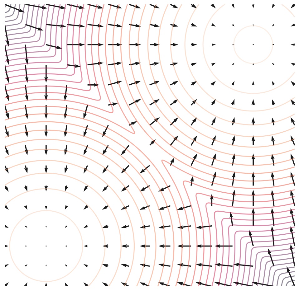
Langevin dynamics提供了一个 MCMC过程，在$p(\mathbf{x})$分布中用得分函数$\nabla_\mathbf{x} \log p(\mathbf{x})$进行采样。

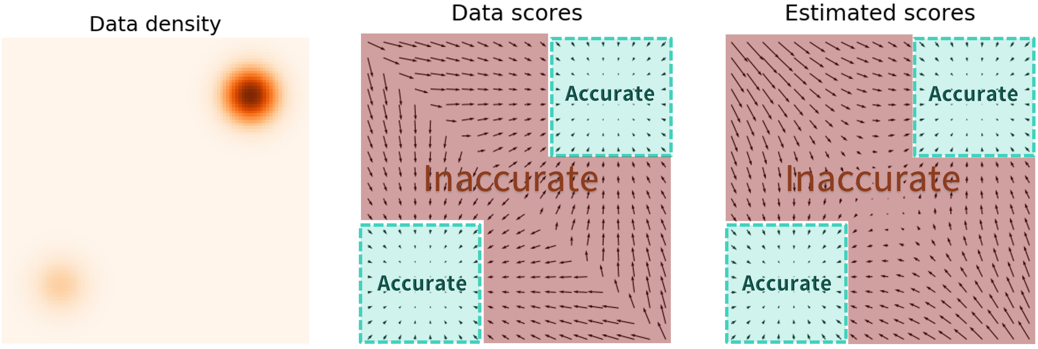
\[\mathbf{x}_{i+1} \gets \mathbf{x}_i + \epsilon \nabla_\mathbf{x} \log p(\mathbf{x}) + \sqrt{2\epsilon}~ \mathbf{z}_i, \quad i=0,1,\cdots, K\]

但在实际训练的时候发现采样的样本很差。究其原因是某些地方样本集较为稀疏, 而estimated scores没有很好的估计（因为$\mathbb{E}{p(\mathbf{x})}[| \nabla\mathbf{x} \log p(\mathbf{x}) - \mathbf{s}\theta(\mathbf{x}) |_2^2] = \int p(\mathbf{x}) | \nabla\mathbf{x} \log p(\mathbf{x}) - \mathbf{s}_\theta(\mathbf{x}) |_2^2 \mathrm{d}\mathbf{x}$, 而$p(x)$在低密度区域值很小。Langevin dynamics采样的时候是先从标准正态分布当中随机采点，这个随机值在概率空间上一般处于样本本身就很少的区域，这就造成了最后的样本不会收敛到期许的概率分布上，从而导致采样的质量很差。

解决这个问题的方法在A connection between score matching and denoising autoencoders初见倪端。

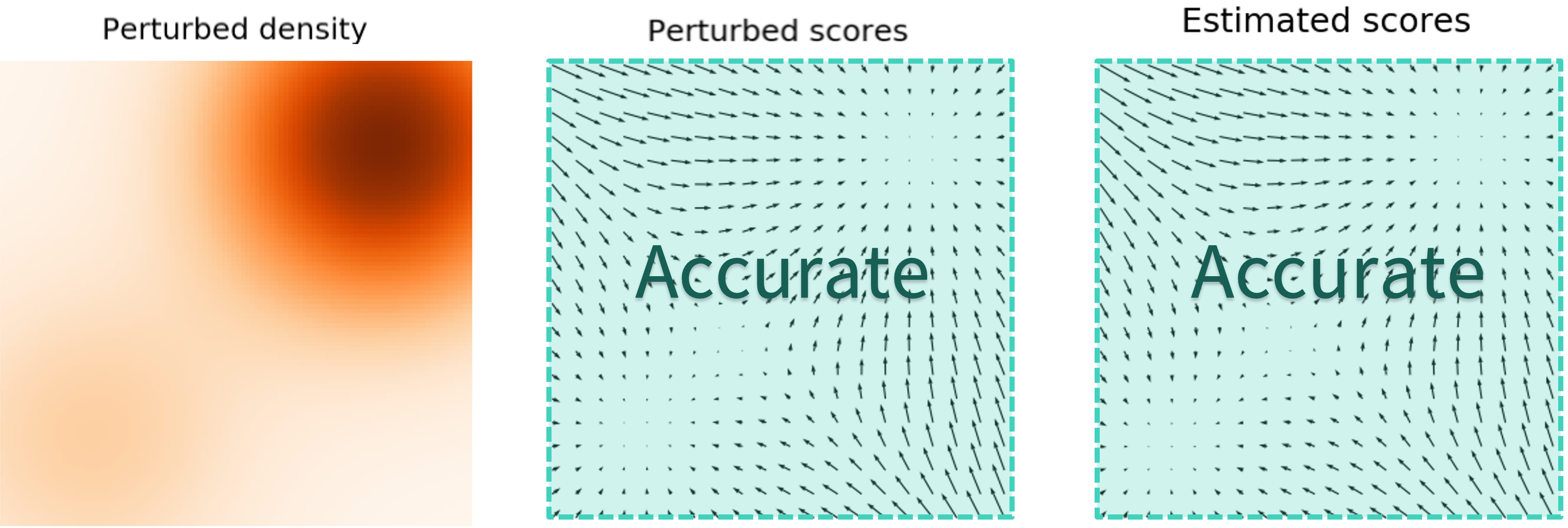
最终的解决方案是用噪声干扰数据点，并在噪声数据点上训练SBM。当噪声幅度足够大时，它可以填充低数据密度区域以提高估计分数的准确性。

那么接下来的问题就是如何加噪声才能使得采样的时候能下降到最有可能的区域了。

在score based models中加入噪声的模型也被称为Noise Conditional Score NetworkGenerative Modeling by Estimating Gradients of the Data Distribution: 同时用不同时间尺度的噪声进行扰动，然后利用annealed Langevin dynamics进行采样。(Improved Techniques for Training Score-Based Generative Models)

假设我们用各向同性的高斯噪声扰动数据，并让标准偏差$\sigma_1 < \sigma_2 < \cdots < \sigma_L$的总数$L$增加。我们首先用每个高斯噪声$\mathcal{N}(0, \sigma_i^2 I), i=1,2,\cdots,L$ 扰动数据分布$p(x)$, 获得了噪声扰动分布：

$p_{\sigma_i}(\mathbf{x}) = \int p(\mathbf{y}) \mathcal{N}(\mathbf{x}; \mathbf{y}, \sigma_i^2 I) \mathrm{d} \mathbf{y}$

也就是说在训练时我们的目标成了$\mathbf{s}\theta(\mathbf{x}, i) \approx \nabla\mathbf{x} \log p_{\sigma_i}(\mathbf{x})$

但是我们无法确认某个噪声尺度是一个合适的噪声尺度，所以我们同时选取$L$个噪声尺度进行训练，此时上式就变成了一个加权：

\[J_{\mathrm{ncsn}}(\theta) = \frac{1}{L} \sum_{l=1}^L \sigma^2 \cdot J_{\mathrm{D}}^{\sigma_l}(\theta)\]

$J_{\mathrm{D}}^{\sigma}(\theta) = \mathbb{E}{p{\mathrm{}}^{\sigma}(\mathbf{\tilde{x}}, \mathbf{x})} \bigg[ \left

\left

\mathbf{s}{\theta}(\mathbf{\tilde{x}}; \sigma) - \nabla{\mathbf{\tilde{x}}} \log p_{\mathcal{N}}^{\sigma}(\mathbf{\tilde{x}}

\mathbf{x}) \right

\right

_2^2 \bigg]$

回顾在DSM中$\nabla \log q_{\sigma}(\hat x)= \frac{-(x-\hat{x})}{\sigma_t^2}$，这里也一样，最终

$J_{\mathrm{D}}^{}(\theta) = \mathbb{E}{p{\mathrm{}}^{}(\mathbf{} \mathbf{x} )}\mathbb{E}_{\tilde{x}} \bigg[ \left

\left

\mathbf{s}_{\theta}(\mathbf{\tilde{x}}; \sigma) + \frac{\tilde{x}-x}{\sigma^2}\right

\right

_2^2 \bigg]$

在训练完NCSN的$\mathbf{s}_\theta(\mathbf{x}, i)$后，我们可以通过$i = L, L-1, \cdots, 1$依次运行 annealed Langevin dynamics来从中生成样本。

此时我们不由得感叹：这个妹妹我曾经见过的！

在DDPM中的时间步长 $t = 1 , 2 ,\cdots,T$ 类似于 NCSN 中不断增加的“噪声尺度”$i = 1,2,\cdots,L$; 两者的回归目标是每个时间步长(或尺度)的噪声向量,学习模型取决于噪声样本和时间步长(或尺度)…

事实上也确实有联系。

connection

在A Connection Between Score Matching and Denoising Autoencoders里揭示了 DSM和去噪自动编码器之间的联系。 DSM中的学习目标可以解释为从损坏样本到真实样本的单位向量，简要来说就是如何对损坏的样本“去噪”，而这正是去噪自编码器所做的。而DDPM 展示了DDPM与NCSN的关系：

在DDPM里我们得到了：

$L_{t-1} - C^\text{} = \mathbb{E}{\mathbf{x}_0, \mathbf{z}} \Big[\frac{ \beta_t^2 }{2 \alpha_t (1 - \bar{\alpha}_t) | } |\mathbf{z}_t - \mathbf{z}\theta(\sqrt{\bar{\alpha}_t}\mathbf{x}_0 + \sqrt{1 - \bar{\alpha}_t}\mathbf{z}_t, t)|^2 \Big]$

而在NCSN中我们得到了：

$J_{\mathrm{D}}^{}(\theta) = \mathbb{E}{p{\mathrm{}}^{}(\mathbf{} \mathbf{x} )}\mathbb{E}_{\tilde{x}} \bigg[ \left

\left

\mathbf{s}_{\theta}(\mathbf{\tilde{x}}; \sigma) + \frac{\tilde{x}-x}{\sigma^2}\right

\right

_2^2 \bigg]$

原文是这样说的

$L_{t-1}$resembles denoising score matching over multiple noise scales indexed by t

训练扩散概率模型的 ELBO 本质上等同于基于分数的生成建模中使用的分数匹配目标的加权组合。

Further more

最初提出noise conditional score-based model的时候，宋博士是相当于直接确定了SDE transition kernel的形式。“设定的不同噪声尺度”是可以变成一个递推的逐步加噪形式的，这个在SDE论文里是有提到的。反观DDPM，虽然定义的是一个递推形式的马尔可夫链，但是训练的时候也是利用transition kernel直接采样加噪的样本的。所以score matching、DDPM、SDE应该是属于统一的框架的

如果我们观察之前的ODE-based model训练，其实可以发现SDE-based model 构建了新方法到传统方法之间的桥梁

summary

自回归网络（Auto-Regressive Networks）
流模型（Flow-based Model）
变分自编码器（Variational AutoEncoder，VAE）

begin with DDPM

"打开了扩散模型的一扇窗"

The import thing behind DDPM

detail of DDPM model

Forward process

Reverse process

score based models

问题提出

connection

Further more

summary

practice

DDPM demo

CATALOG

FEATURED TAGS

FRIENDS